Modeling Data

NBA MVPs data analysis from 1955 all the way up to 2019

We learned about the basics of R programming and I want to finish my knowledge sharing by going over one of the projects that I very much enjoyed analyzing data with R programming features. 

I will try to explain the details of the project below with the important points through this post. There is some new functions that we will look into. In my first availability, I would like to explain more details in a video.

I love sports and basketball is one of them.  I had a data source that shows NBA (National Basketball Association) MVPs (Most Valuable Players) from 1955 all the way up to 2019. In this data set, some of the categories are games, play minutes, points total (PTS), rebounds, assists, steals, and etc. I wanted to analyze this data and get the answers for the following two questions;

What factors are most important to win MVP? 

Who is the all-time most efficient MVP?

Data file looks like the following;

Project codes – Overview 

Let’s go over project sections; 

Section 1

Importing data set, getting a summary of four categories which I thought are most important, then I view the data afterwards to make sure all the variables are present in, nothing’s missing and I also do the same to make sure there is no NA (none applicable) in any column either. Data is in a csv file and named as NBA_Improve.csv. 

********************************************************

#Importing the data set

data=read.csv(“C:\\csv\\NBA_Improve.csv”,header=TRUE)

#Question:What factors are most important to win MVP?

#Question:Who is the all time most efficient MVP?

#Summarized the data’s file and variables

summary(data)

summary(data$PTS)

summary(data$Assists)

summary(data$Minutes.Played)

summary(data$Total.Rebounds)

#To view data set 

View(data)

#To make sure that all variables are there

data[!is.na(data$Minutes.Played),]

#To check if there is any NA

data[is.na(data$Steals),]

#No need to insert na.string for no NA detected in variables only in co-variables

***************************************************************

Section 2

Installing packages so I can make the plots and run data set more smoothly. I included a couple of packages as you can see below and then all of these are installed into the library.

**************************************************************

#library 

#Need to install packages to make plots and data set to run smoothly

install.packages(“lme4”)

#Which includes lmer

install.packages(“splines”)

install.packages(“ggplot2”)

install.packages(“quantreg”)

install.packages(“insight”)

#To make sure that the packages are installed in the library

library(“lme4”)

library(“splines”)

library(“ggplot2”)

library(“quantreg”)

library(“insight”)

********************************************************************

Section 3

Plotting out different types of graphs (bar, scatter and quantile graphs). I analyzed each one to check the relationship between plotted data and together between graphs.

***********************************************************************

#Using ggplot to graph data

#Graph 1 colored bar graph

ggplot(data=data, aes(x=Season,y=PTS, fill=Player)) + geom_bar(stat=”identity”)+coord_flip()+geom_text(aes(label=Player),nudge_y=-8)+theme(axis.text.x = element_text(angle=90))

#Graph 2 colored scatter plot

ggplot(data=data) + geom_point(mapping = aes(x = Player, y = Minutes.Played, color=PTS),size=4)+theme(axis.text.x=element_text(angle=90))

#Graph 3 colored scatter plot

ggplot(data=data) + geom_point(mapping = aes(x = Player, y = Minutes.Played, color=Assists),size=4)+theme(axis.text.x=element_text(angle=90))

#Graph 4 quantile graph

ggplot (data=data, aes(Total.Rebounds,Player))+geom_point(size=4)+geom_quantile(quantiles=1)

***********************************************************************

Section 4 

Analyzing data with different hypotheses and finding answers for questions.   In this section, I used anova model/function. Let’s quickly look at it;

What is anova?

Anova stands for Analysis of Variance and it is another statistical technique that is used to test the hypothesis (measure statistical difference) if you have more than two or more group means (group by one or more variables) could be obtained from the same populations.  In this post,  I will only go through implementing it with one way anova based on the linear model (lmer function). 

One way anova

In one way anova, we have one independent variable with more than two (a least three) levels and one dependent variable.  For example;  independent variable is fruits and we have data for apple, pear, banana (groups). We want to find out what is the difference in the price of 1 lb (or kg), dependent variable. 

Data preparation is also very important.  Make sure you have NA data in any column of the data set. 

We can create different hypotheses.  The null hypothesis means there is no difference between group means.  The other alternative hypothesis means, at least one group differs from the mean of the dependent variable. 

Let’s understand first what is variance (residual) and move forward to section 4 set up after that.

Variance (residual) is a measure of variation of values or in other word, discrepancy between different data.  Higher percentage of variance means stronger strength.  It is represented with R², coefficient of determination, if you are doing a regression analysis. 

In the following section 4 codes,  you will see 4 different hypotheses. In section 1,  we loaded the lme4 package.  That provides functions to fit and analyze linear models. I used the lmer function from that package to fit a linear mixed effect model to each hypothesis data (it is also called lmer test) via REML (logical scalar, default is TRUE).

REML stands for restricted maximum likelihood and FALSE is used if comparing data with different fixed effects, TRUE (default, no need to write it in code) is used if comparing data with different random effects).

The flowing coding has different sections to analyze and calculate the R² data for each hypostases.

************************************************************************

#Anova checking the hypotheses

#Null hypothesis

data.null = lmer(PTS ~ (1|Player), data=data, REML=FALSE)

#Alternative hypothesis M1

data.M1 = lmer(PTS ~ (1|Player) + Minutes.Played, data=data, REML=FALSE)

#Alternative hypothesis M2

data.M2 = lmer(PTS ~ (1|Player) + Assists, data=data, REML=FALSE)

#Alternative hypothesis M3

data.M3 = lmer(PTS ~ (1|Player) + Minutes.Played + Assists, data=data, REML=FALSE)

#Summary of data

summary(data.null)

summary(data.M1)

summary(data.M2)

summary(data.M3)

#One-way Anova

anova(data.null,data.M1)

anova(data.M1,data.M2)

anova(data.null,data.M3)

#Hypothesis residuals plots

plot(data.null, main = “Null hypothesis”, xlab = “Fitted Values for points per player”, ylab = “Residuals”)

plot(data.M1, main = “Hypothesis M1”, xlab = “Fitted Values for points per player with minutes played”, ylab = “Residuals”)

plot(data.M2, main = “Hypothesis M2”, xlab = “Fitted Values for points per player with assists”, ylab = “Residuals”)

plot(data.M3, main = “Hypothesis M3”, xlab = “Fitted Values for points per player with minutes played and assists”, ylab = “Residuals”)

#R^2 values calculation – the conditional R^2 is the fixed+random effects variance divided by the total variance, and indicates how much of the model variance is explained by your complete model

#var.fixed – variance with fixed effect

#var.random – variance of random effect

#var.residual-residual variance (sum of dispersion)

varsn<-insight::get_variance(data.null)

r2_conditionaln <- (varsn$var.fixed + varsn$var.random) / (varsn$var.fixed + varsn$var.random + varsn$var.residual)

print(r2_conditionaln)

varsn_1<-insight::get_variance(data.M1)

r2_conditionaln_1 <- (varsn_1$var.fixed + varsn_1$var.random) / (varsn_1$var.fixed + varsn_1$var.random + varsn_1$var.residual)

print(r2_conditionaln_1)

varsn_2<-insight::get_variance(data.M2)

r2_conditionaln_2 <- (varsn_2$var.fixed + varsn_2$var.random) / (varsn_2$var.fixed + varsn_2$var.random + varsn_2$var.residual)

print(r2_conditionaln_2)

varsn_3<-insight::get_variance(data.M3)

r2_conditionaln_3 <- (varsn_3$var.fixed + varsn_3$var.random) / (varsn_3$var.fixed + varsn_3$var.random + varsn_3$var.residual)

print(r2_conditionaln_3)

***************************************************************************

Looking into plots and calculations 

Looking at the summary data, I analyzed the data statistics for each variables.

I created four plots like following;

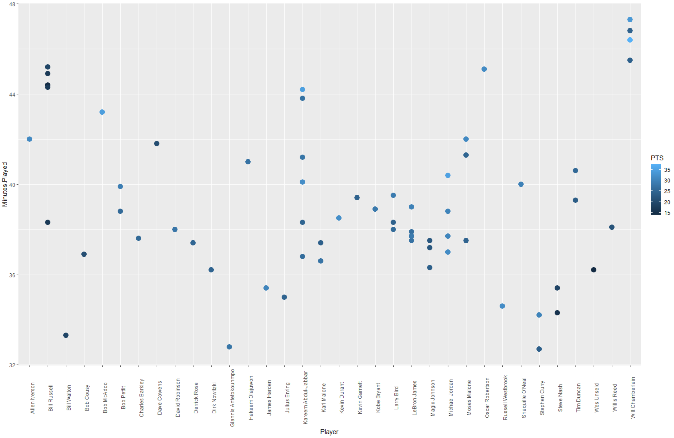
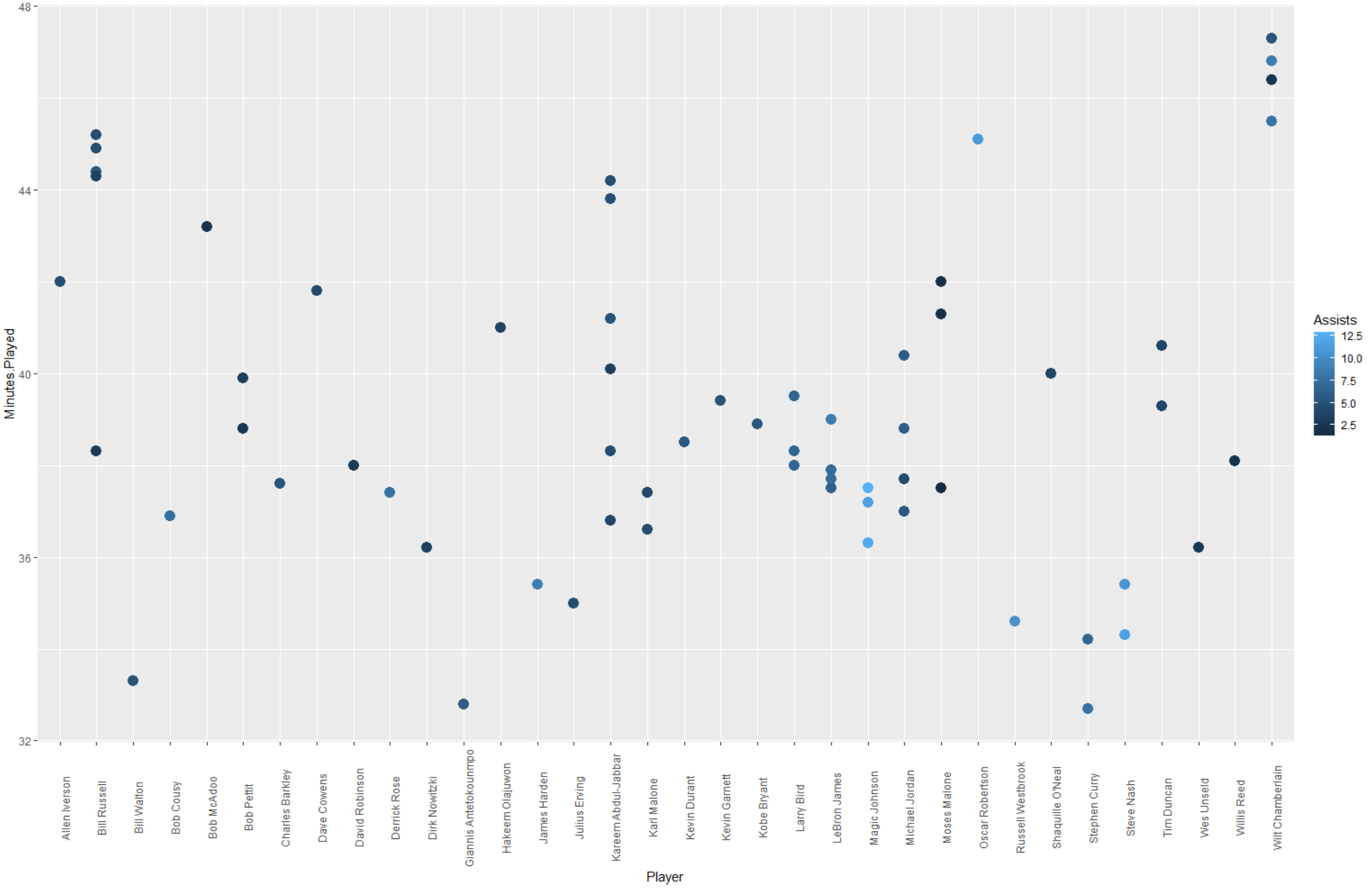
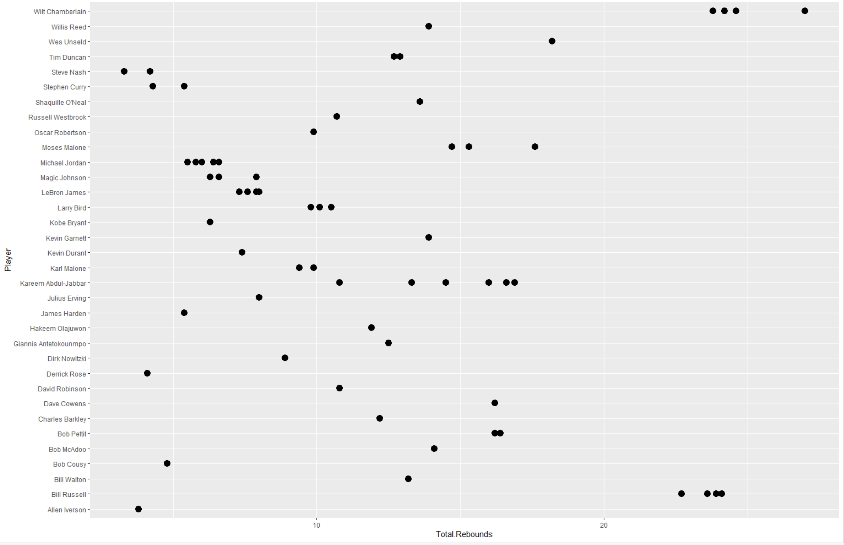
Based on those plots, I understand that who score the most points, who score the most points with time, who got the most assist with time and lastly what is the total rebound per player.

Next, I created four hypothesis, plotted each hypothesis residual plot and calculated R² for each hypothesis.

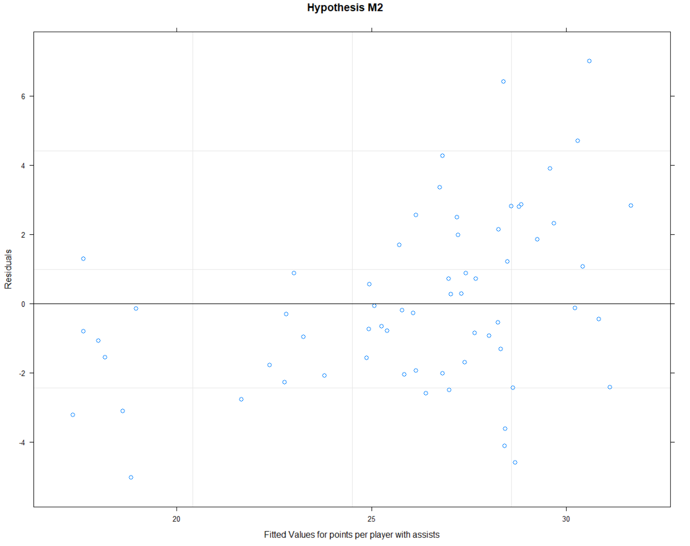
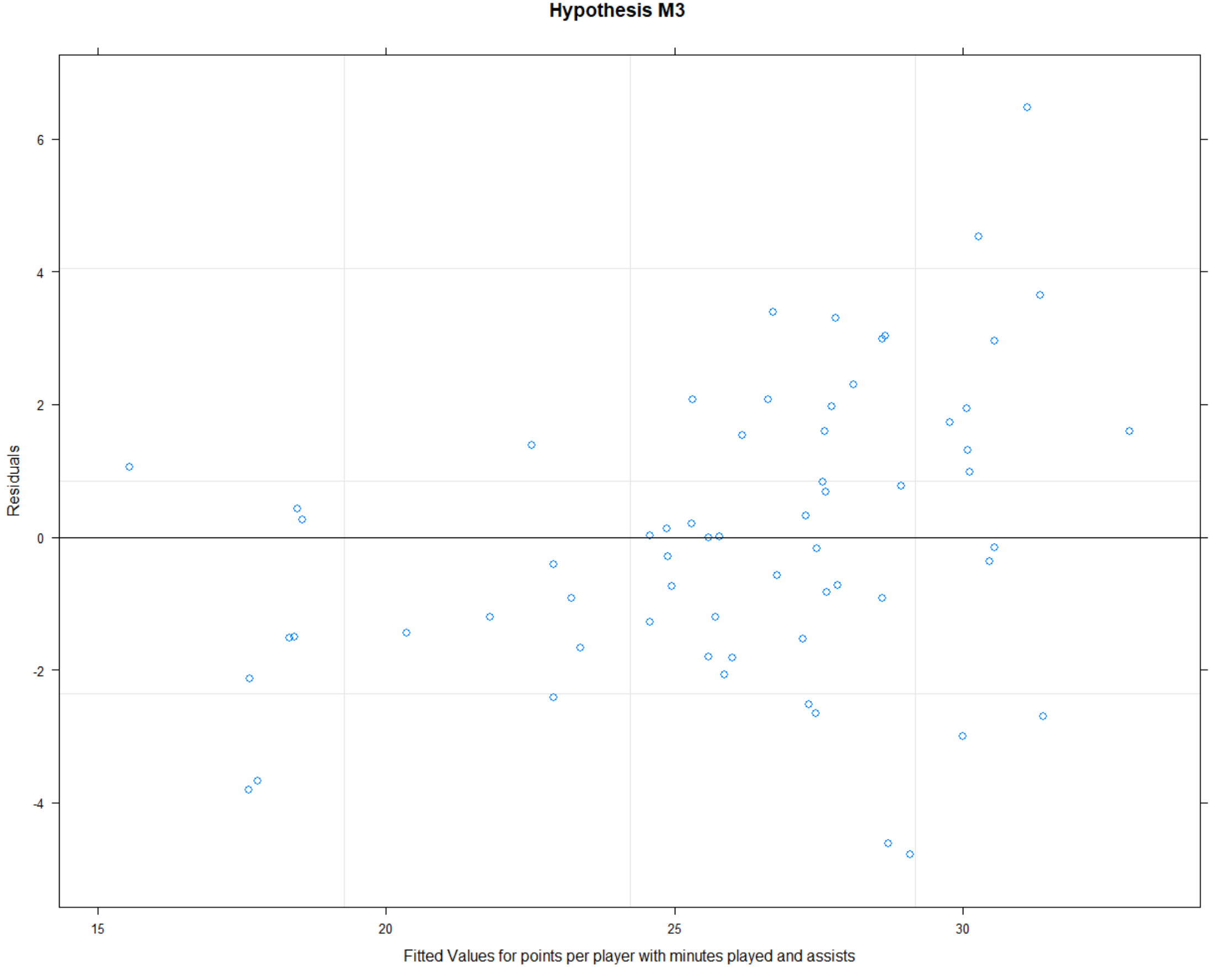
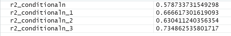
Based on the calculated R² values, I understand that hypothesis 3 is the most accurate and shows me which data are most important.

Answers to questions

Based on data analysis, following is the conclusion for each question;

What factors are most important to win MVP? 

The most important factors are points, minutes played and assists.

Who is the all-time most efficient MVP?

The most efficient MVP of all time was Russel Westbrook. Because, he was able to get most points and assists with less minutes played time then the others.

We are concluding R programming with this post and going to start learning Java programming starting from the next post. I hope you have a basic understanding about R programming now and looking forward to learning more.

If you want to get full project codes,  please go to the Projects and click on R project.